Training Compute-Optimal Large Language Models
Hoffmann et al., arXiv:2203.15556
Paper Abstract
We investigate the optimal model size and number of tokens for training a transformer language model under a given compute budget. We find that current large language models are significantly undertrained, a consequence of the recent focus on scaling language models whilst keeping the amount of training data constant. By training over 400 language models ranging from 70 million to over 16 billion parameters on 5 to 500 billion tokens, we find that for compute-optimal training, the model size and the number of training tokens should be scaled equally: for every doubling of model size the number of training tokens should also be doubled. We test this hypothesis by training a predicted compute-optimal model, Chinchilla, that uses the same compute budget as Gopher but with 70B parameters and 4× more data. Chinchilla uniformly and significantly outperforms Gopher (280B), GPT-3 (175B), Jurassic-1 (178B), and Megatron-Turing NLG (530B) on a large range of downstream evaluation tasks. This also means that Chinchilla uses substantially less compute for fine-tuning and inference, greatly facilitating downstream usage. As a highlight, Chinchilla reaches a state-of-the-art average accuracy of 67.5% on the MMLU benchmark, greater than a 7% improvement over Gopher.
Problem
- Under a fixed FLOPs budget, how should you trade off model size \(N\) vs number of training tokens \(D\)?
- They model final pretraining loss \(L(N, D)\) as a function of parameter count \(N\) and token count \(D\). The optimal pair \((N, D)\) describes how to allocate compute \(C\) (subject to the paper’s FLOPs model, roughly proportional to \(N \times D\) for training).
Data and scale
- Empirical estimates come from 400+ models, from under 70M to over 16B parameters, trained on ~5B to 400B+ tokens.
- Chinchilla: a compute-optimal ~70B model trained on ~1.4T tokens. Beats the much larger Gopher. The smaller \(N\) also lowers inference cost.
The paper uses three approaches. In all cases they train many models with different \(N\) and \(D\) and use training curves / final losses to fit how \(N\) and \(D\) should scale with compute. The three methods agree: \(N_{\mathrm{opt}} \propto C^{a}\) and \(D_{\mathrm{opt}} \propto C^{b}\) with \(a \approx b \approx 0.5\), which is very different from Kaplan et al.
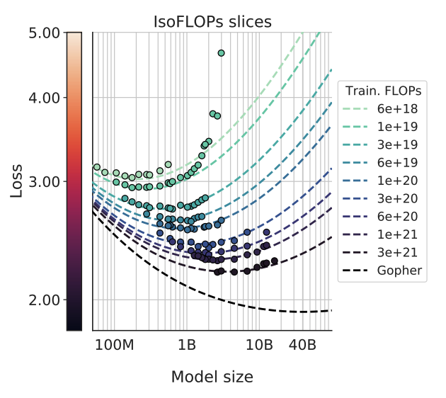
This figure illustrates the optimal model size for lowest loss for any given pretraining FLOPs budget. The valley shows the optimal model size to achieve lowest loss. Left side of the valley is not ideal - the model is too small for the budget. Right side of the valley is also not ideal - the model is too large and you ran out of compute on the training tokens side.
Approach 1 — Fix model sizes, vary training tokens
For a fixed family of model sizes (about 70M–10B+ params), train each size for several training horizons (four cosine lengths spanning a 16× range in tokens). Smooth/interpolate training loss vs FLOPs per run; at each FLOP level, pick the \((N, D)\) pair with lowest loss. Fit power laws \(N_{\mathrm{opt}} \propto C^{a}\), \(D_{\mathrm{opt}} \propto C^{b}\) to the resulting frontier (\(a \approx 0.50\), \(b \approx 0.50\)).
Approach 2 — IsoFLOP profiles
For nine fixed training-FLOP budgets, sweep model size (up to 16B here) and set \(D\) so total training FLOPs matches each budget. Plot final loss vs \(N\) at fixed FLOPs; you get a valley—optimal \(N^{*}\) per budget. Fit a parabola to each iso-FLOP curve to locate the minimum, then again fit \(N_{\mathrm{opt}}\) and \(D_{\mathrm{opt}}\) vs compute (\(a \approx 0.49\), \(b \approx 0.51\)).
Approach 3 — Parametric loss \(\hat{L}(N, D)\)
Fit all final losses from Approaches 1 & 2 with a parametric form
\[\hat{L}(N, D) = E + \frac{A}{N^{\alpha}} + \frac{B}{D^{\beta}}\](first term is irreducible error, second is underparameterization, third term is finite data), via Huber loss on log-loss. Then minimize \(\hat{L}\) subject to \(\mathrm{FLOPs}(N,D) \approx 6ND\) to get the compute optimal frontier in closed form; exponents come out \(a \approx 0.46\), \(b \approx 0.54\)—still near 50/50 for \(N\) vs \(D\).
vs Kaplan scaling laws
- Kaplan et al. (prior “scaling laws” narrative): suggested \(N\) should grow much faster than data for a given compute budget.
- This work: refined power-law fits and found that \(N\) and \(D\) should scale in roughly equal proportion as compute grows (for every doubling of model size, about double the tokens as well).
- Implication: many models at the time were under-trained; model size was too large for how much data they saw.
Takeaways and Questions:
- Authors found that given a fixed training compute, amount of training tokens should be approximate 20x the model size. So for a 1B model, optimal training tokens is around 20B.
- However this is only for training compute, and doesn’t account for inference compute. If a model serves many users it can be good to overtrain the model, like 50x or 100x, so the smaller model is cheaper to serve.
- How can we rewrite the 3D scaling law \((N,D,R)\) to optimize for total life-cycle compute rather than just training compute?